If we postulate that the arrangement of life in the ocean results from the interaction between the ecological niche (sensu Hutchinson) of species and the fluctuations in the environmental regime, we can predict a number of spatial and temporal patterns at different organisational levels ranging from the species to the biospheric level and at different spatial and temporal scales.
At the species level, the METAL theory enables the understanding of space and time responses of species to environmental changes at many scales of variability. Niche shape can be modelled by using many different functions (Figure 1). Some researchers have used a trapezoidal (Kaschner et al. 2008) or a rectangular niche (Beaugrand et al. 2013b), the latter being used when only presence/absence are considered (Figure 1, panels b-c). The niche can be symmetric (Figure 1, panels a-d) or asymmetric (Figure 1, panels e-f). The consideration of asymmetry is important for some species as many ectotherms seem more sensitive to warming than cooling (Araujo et al. 2013).
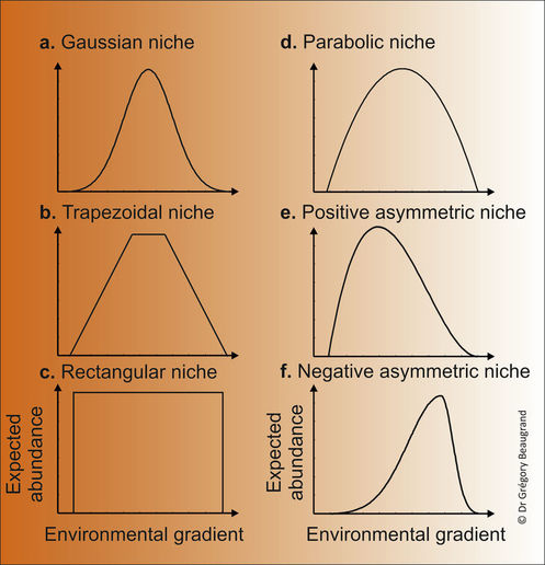
Figure 1. Examples of niche shape that can be used as part of the METAL theory. a. Gaussian niche. b. Trapezoidal niche. c. Rectangular niche. d. Parabolic niche. e. Negative asymmetric niche. f. Positive asymmetric niche. From Beaugrand (in preparation).
Below we model the niche of a species using a Gaussian function (Ter Braak 1996) and a single environmental parameter: mean Sea Surface Temperature (SST). The response curve of the abundance E of a pseudospecies s in a given site i and time j to change in SSTs was modelled as follows:
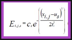
With Ei,j,s the expected abundance of a pseudospecies s at location i and time j; cs the maximum value of abundance for species s (here this was fixed to one); xi,j the value of temperature at location i and time j; us the thermal optimum and ts the thermal amplitude for species s. The thermal tolerance is an estimation of the breadth (or thermal amplitude) of the species thermal niche (or bioclimatic envelope) (Ter Braak 1996).
1. Species spatial distribution
We first start by estimating species spatial distribution, a currently active area of research based on the application of Ecological Niche (ENM) or Spatial Distribution (SDM) Models (Albouy et al. 2012; Araujo and Guisan 2006; Cheung et al. 2008; Lenoir et al. 2011; Raybaud et al. 2013). As temperature is a fundamental parameter, we use a thermal niche for simplification. However, the METAL theory should use the full multidimensionality of the niche; for example, light limitations probably take place in high-latitude regions (Mitchell et al. 1991; Sverdrup 1953), influencing the spatial distribution and the phenology of some species (Edwards and Richardson 2004), and oxygen limitation may be important in some oceanic regions such as the East Pacific or the Indian Oceans (Hofmann et al. 2011).
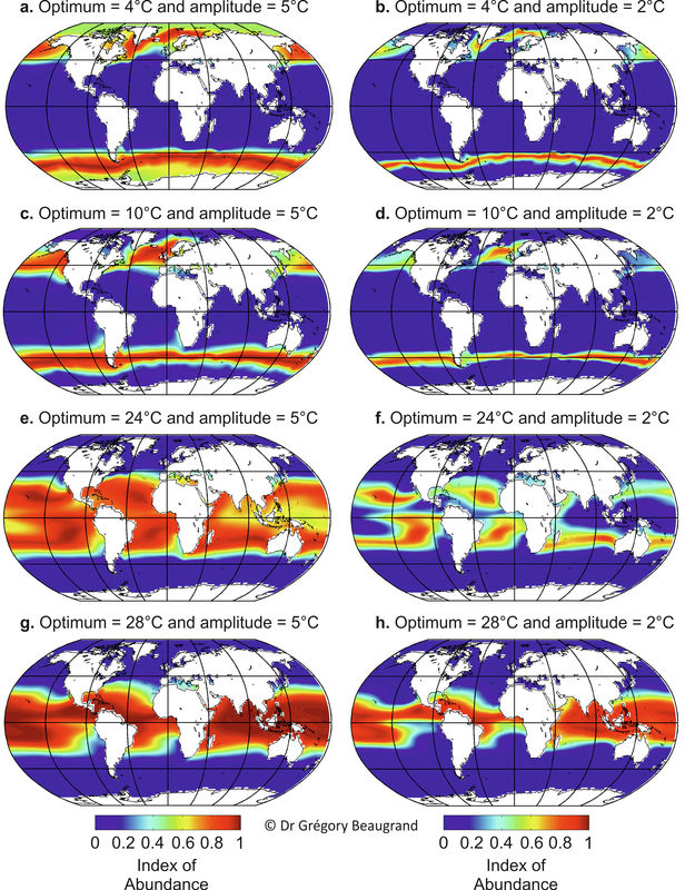
Figure 2. Probability of occurrence of some pseudo-species having a Gaussian niche with different thermal optima and amplitude. Within a map, different areas characterized by a high probability of occurrence can be occupied by different pseudo-species according to Buffon’s Law (see main text). From Beaugrand (in preparation).
We created hypothetical species characterized by a Gaussian thermal niche with 4 different values of us for 2 values of ts (Fig. 2 and 3). Figure 2 shows the probability of species occurrence based on a given thermal niche. Even if similar environmental (here, thermal) conditions occur in different oceanic and neritic regions, different species may be present according to Buffon’s Law, also known as the first principle of biogeography (Lomolino et al. 2006). We therefore designed an algorithm that enables species characterised by the same thermal niche and that are spatially separated to be differentiated. In practice, when an area with high contiguous probabilities (i.e. above 0.4) was separated by at least one geographical cell (the spatial grid was 2°x2°) from another contiguous area with high probabilities, the two areas were considered to be occupied by two different species having the same thermal niche. Figure 3 shows the results of the application of this algorithm on data displayed in Figure 2, each colour representing a different species in each map. The consideration of a different threshold did not lead to a different conclusion.
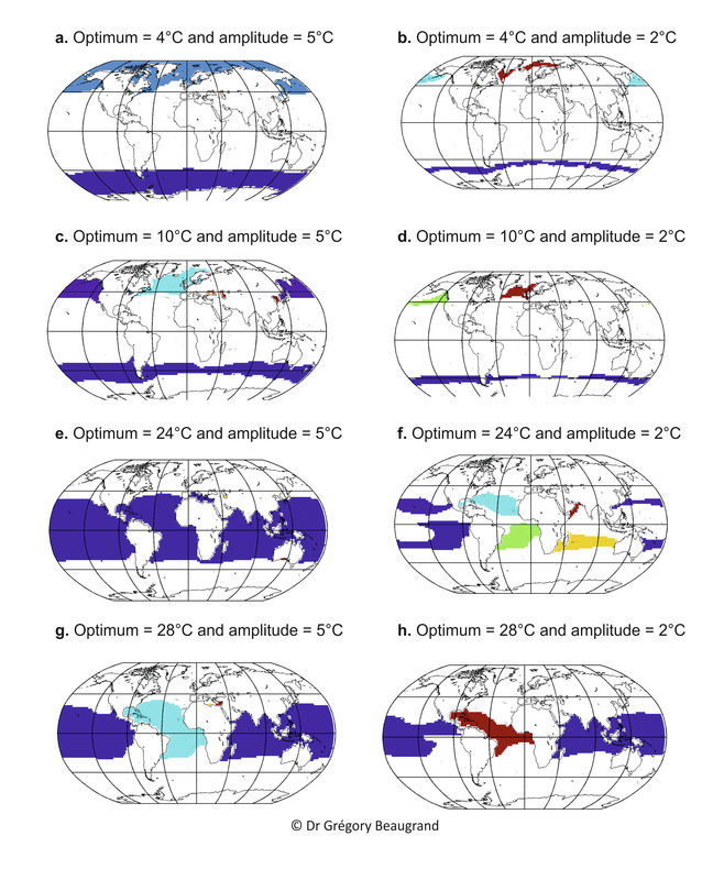
Figure 3. Spatial distribution of some pseudo-species having a Gaussian niche with different thermal optima and amplitudes. Within a map, when an area with high contiguous probabilities of occurrence above 0.4 (see Fig. 2) was separated by at least one geographical cell (the spatial grid was 2°x2°) from another contiguous area with probabilities higher than 0.4, the two areas were considered to be occupied by two different species having the same thermal niche. Within a map, each pseudo-species (with the same niche) is represented by a different colour. From Beaugrand (in preparation).
A universal eurythermic species is the only species than may have a pandemic distribution (not shown). Other species with a smaller degree of eurythermy will exhibit a more restricted distributional range. Many species are likely to exhibit a circum-oceanic (e.g. circum-polar and circum-temperate) distributional range (Fig. 2-3a-e for both hemispheres and 2-3c-d for the Southern Hemisphere exclusively). By either considering more ecological variables (e.g. bathymetry, oxygen concentration, macro-nutrients and micro-nutrients) or in the case of stronger stenoecy (see Figure 2-3a versus Figure 2-3b and Figure 2-3e versus Figure 2-3f), the circum-oceanic distributions are likely to fade and to become more fragmented (i.e. disjointed distribution).
Tropical/warm-temperate species (Figure 2e-h) are less likely to have a circum-oceanic distribution because of the presence of continents that act nowadays as geographical barriers. However, this figure also depends on the degree of euryoecy (Figure 2-3e versus Figure 2-3f). Stenothermic tropical/temperate species occurring in both hemispheres (Figure 2f) may also become isolated enough at the equator to become different species (allopatric speciation). Such an equatorial diminution can be permanent or not.
The METAL theory may help to understand better the relationship between the niche of a species and its spatial distribution. Lomolino and colleagues (Lomolino et al. 2006) stated that the geographical range of a species reflects its ecological niche. This also explains the relative success of ecological niche modelling, which enables from the modelling of species’ ecological niche to not only infer their past and current spatial distribution but also to project their future spatial range from the knowledge of forthcoming environmental conditions (Lenoir et al. 2011; Raybaud et al. 2013). Such a modelling approach has lacked however a theoretical framework to be better understood and accepted by all scientists. Brown’s theory (Brown 1984) links species’ local density and range with species’ ecological niche. Although this seems to be the case in general (Beaugrand et al. 2014b), this relationship can sometimes be not so straightforward. Some species can have a more restricted range (and sometimes be endemic) because of the presence of geographical barriers (e.g. landmass; see Figure 3c and Figure 3f). For example, despite that all species have the same niche, we can see in Figure 3f that one has a very limited spatial distribution in the northern part of the Indian Ocean because of the presence of the Eurasian continent. Such a restricted spatial distribution, modulated by the realised environment (Jackson and Overpeck 2000), may substantially affect the modelling of the niche by ENMs. A high level of endemism seems therefore possible in the Mediterranean Sea (Figure 3c, e, g), a pattern frequently reported in the literature (Lasram et al. 2010).
Studies have shown that the METAL theory explains of large proportion of the variance of the spatial distribution of some species (Beaugrand et al. 2014b). For example, by considering annual SST, bathymetry, chlorophyll a and photosynthetically active radiation, the modelled spatial distribution of the calanoid copepod Calanus finmarchicus was close to the spatial distribution observed from the Continuous Plankton Recorder (CPR) survey (Figure 4). Approaches based on ENMs often successfully reconstruct marine species spatial distribution (Beaugrand et al. 2011; Lenoir et al. 2011; Raybaud et al. 2013; Rombouts et al. 2012). ENMs have been more criticised in the terrestrial realm but this might be related to the higher heterogeneity of this realm and the strong direct influence of human activities.
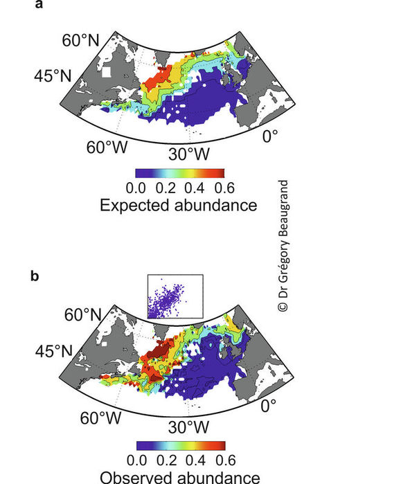
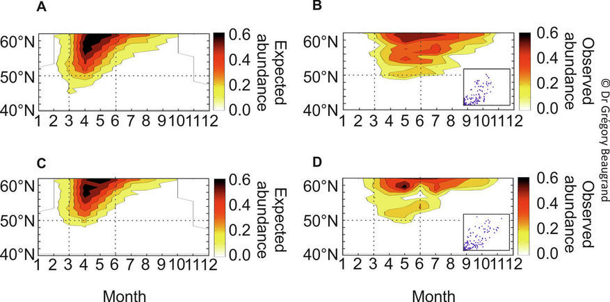
Figure 4. Expected (a) and observed (b) mean spatial distribution of the calanoid copepod Calanus finmarchicus. Observed data were from the Continuous Plankton Recorder (CPR) survey (Reid et al. 2003). Expected abundance was calculated using the Non-Parametric Probabilistic Ecological Niche (NPPEN) model based on 4 ecological dimensions (see text). The scatterplot shows the relationships between expected and observed abundance of C. finmarchicus. From Beaugrand and colleagues (Beaugrand et al. 2014b).
2. Spatial distribution and phenology
Phenology (i.e. the study of periodic biological phenomena), is expected to be altered as climate changes. Processes behind phenological shifts are complex but temperature is often advocated in both the terrestrial and the marine realms (Root and Hughes 2005). For example, phenological shifts in many planktonic species (e.g. dinoflagellates and copepods) have been reported in the North Sea (Edwards and Richardson 2004) and attributed to regional warming. Mackas and colleagues (Mackas et al. 2012) in a review of phenological shifts in different oceanic systems also proposed temperature as the main driver, although it was apparent that other factors (e.g. day-length, mixed-layer depth) may play a significant role (Edwards and Richardson 2004). Biogeographical movements, also termed species tracking (Peterson et al. 2005), are often seen as latitudinal species shifts in response to regional warming (Beaugrand et al. 2002; Parmesan and Yohe 2003; Perry et al. 2005; Thomas and Lennon 1999). In the marine realm, biogeographical shifts have taken place, consistent with latitudinal changes expected under climate warming and hydro-climatic variability. For example, in the north-east Atlantic a poleward movement of warm-water calanoid copepods has been associated with concomitant northward retraction of cold-water species (Beaugrand et al. 2002) and similar biogeographical movements have been observed in both exploited and unexploited fish (Brander et al. 2003; Perry et al. 2005). How both phenological and biogeographical shifts may be connected? And by which mechanisms?
Let’s first work on a simple case, where the niche is one-dimensional and only represented by SST, to establish at the species level the theoretical foundations between species niche, species spatial distribution and phenology. The response curve of the abundance E of a pseudospecies s in a given site i and time j to change in SSTs can be modelled using the equation presented above.
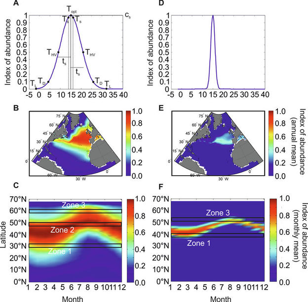
Figure 5. Theoretical relationships between species distribution, latitudinal range and phenology of two cold-water species: one eurytherm and one stenotherm. Theoretical thermal niche of an (A) eurytherm and (D) a sternotherm. For meaning of Topt, Ts, THV, TD and TL see Fig. 11.8 and text. Theoretical mean annual spatial distribution of (B) eurytherm and (E) stenotherm species. Theoretical changes in abundance as a function of latitudes and months for (C) eurytherm and (F) stenotherm species. Zone 1: part of the distribution where seasonal maximum occurs in spring/winter. Zone 2: part of the distribution where seasonal extent is highest. Zone 3: part of the distribution where seasonal maximum is located at the end of summer. From Beaugrand and co-workers (Beaugrand et al. 2014a).
Using only the thermal dimension of the niche as an example, we modelled the expected mean annual distributional range of a hypothetical temperate species with a broad thermal niche (Figure 5A; thermal optimum us=15°C and thermal tolerance ts=5°C). For this pseudospecies (Figure 5A), the METAL theory predicts a mean annual extratropical range with a poleward limit to the south of the Polar Biome and an equatorward limit north of the Atlantic Trade Wind Biome (Longhurst 2007) (Figure 5B). The calculation of the expected species’ abundance as a function of latitude and month leads to three predictions relating latitudinal range and phenology (Figure 5C). First, in the southern part of its distributional range (zone 1; Figure 5C), the organism has a seasonal maximum in winter or spring, the latter period is more likely when ecological factors such as Photosynthetically Active Radiation (PAR) affect the species either directly through its influence on photosynthesis (e.g. phytoplankton), or indirectly through trophodynamics (e.g. herbivorous zooplankton). PAR influence on primary production is prominent polewards (Behrenfeld 2010). At its southern range, such a species could not adjust its phenology in response to an increase in sea temperature, resulting in a local reduction of its annual mean and a northward biogeographical shift. Both the resistance and the resilience of this cold-water species to warming are expected to be small, but the opposite is expected in the case of a cooling. Second, at the centre of its range (zone 2; Figure 5C) the species will exhibit its maximum seasonal extent, the duration being modulated by the breadth of its thermal niche ts (here, the species can occur all months of the year, so long as other niche dimensions such as PAR or Length Of Day (LOD) do not exert a controlling influence). Here, sea warming is expected to trigger a shift towards an earlier phenology. All else being equal or held constant, erosion of the seasonal occurrence period in late summer should be compensated at an annual scale by higher abundance towards spring or early summer and consequently, no substantial alteration in annual species abundance is expected; species resistance and resilience to warming are greatest in this area. Third, at the northern edge of its distributional range (zone 3; Figure 5C), the species is likely to peak in summer or late summer. In this case if temperatures warm, the cold-water species can extend its occurrence in early summer and spring, resulting in an increase of its annual mean abundance. If SST warms north of its northern boundary, a northward range shift will occur although first occurrences are likely to be detected first in late summer when sea temperatures are highest.
In the case of a theoretical stenotherm (thermal optimum us=15°C and thermal tolerance ts=1°C), the thermal sensitivity increases and the overall species’ abundance declines (Figure 5D-E versus Figure 5A-C). Although the same phenological pattern is expected in its poleward and equatorward distributional range, this species does not occur throughout the year at its range center (Figure 5F). In this case, Zone 2 (Plate 11.3F) will be narrow and the species will persist for fewer months. It follows that a stenotherm will react quickly to an increase in temperature even at the center of its range. The stenotherm is therefore expected to be more sensitive to a climate-mediated shift in temperature. Predictions can be established for other species (e.g. tropical species).
Comparing the two theoretical species, local density of the eurytherm is much higher than the stenotherm (Figure 5). This result is in agreement with the Brown’s theory (Brown 1984) that relates the local density of a species to the size of its spatial distribution and its ecological niche; this implies that a stenotherm should have both a lower local density and a smaller spatial range, as predicted by the METAL theory. Although Brown’s theory, which holds true for many marine organisms (Sunday et al. 2012), was exclusively proposed to explain the relationship between niche breadth and distributional range, our results indicate that the species ecological niche can also explain how species and communities will respond to changes in temperature in time and space.
3. Phenological and biogeographical shifts
We tested the METAL theory against real data for marine species, choosing the marine copepod Calanus finmarchicus (Beaugrand et al. 2014a). The niche was modelled using the Non-parametric Probabilistic Ecological Niche (NPPEN) model (Beaugrand et al. 2011), which calculated the expected abundance of C. finmarchicus as a function of monthly SST, monthly PAR, monthly chlorophyll-a concentration and bathymetry. These four parameters form the most important niche dimensions for C. finmarchicus (Helaouët and Beaugrand 2009; Reygondeau and Beaugrand 2011). Seasonal changes in PAR are highly correlated positively with Length of Day, which has been assumed to be an important controlling factor of the initiation and termination of C. finmarchicus diapause (Fiksen 2000). As NPPEN is non-parametric, the niche was not Gaussian in contrast to the example developed previously.
When the expected abundance of C. finmarchicus is represented as a function of latitude and month (1960-1979, a relatively cold period (Beaugrand et al. 2008); Northeast Atlantic between 30°W and 10°W), the model predicts that (1) the species should have a seasonal maximum in spring at the southern edge and (2) between spring and summer towards the centre of its spatial distribution (Figure 6A).